1. Introduction
Reliable information about the life of electro-mechanical components is very important to the design of new products. Today manufacturers face market challenges to launch innovative products with significant new content in shorter times. To do so, they must rely on estimates of component’s life to establish warranty periods and after sales services. Reliable life information is also necessary to customers, since they rely on Life Cycle Cost (LCC) analysis to define their own maintenance strategy, particularly for critical systems in the manufacturing context (MIL-HDBK, 1997).
Information about reliability of components and systems usually comes from three basic sources, namely the manufacturer’s specifications, field data about performance of components under warranty and experiments performed during new products development. Although useful in some sense, all of them have drawbacks.
Component’s life data from manufacturers do not cover all possible use conditions for new products. Therefore, further efforts are needed to come up with the desired information under the specific and new operational conditions (Escobar and Meeker, 2006). Data about components performance in field is not readily available for high-end products that by design are intended to have few or non-failures during warranty. Therefore, it demands long periods to gather the warranty data besides special management and data analysis approaches to validate the information (Marcorin and Abackerli, 2006; Wu, 2012). Finally, experiments are usually time and resources consuming if executed under normal working conditions, demanding therefore special approach to allow having the needed information during the development phase of a new product.
Under these circumstances, Accelerated Life Testing (ALT) is useful in identifying better designs, materials and major component’s characteristics due to their shorter testing times through new products development (Escobar and Meeker, 2006), particularly when focusing on better understanding of expected failure modes and checking life estimates (Huang et al., 2007).
However, to successfully collect data from ALT tests there are some experimental care to be taken to guarantee the reliability, the adequacy and the validity of test results (Escobar and Meeker, 2006). Experimental tests always have their inherent measurement uncertainties, which require fine-tuning of the experimental setup to agree with the theoretical conditions assumed during the experiment design. Moreover, most of the relevant literature on experimental life testing and analysis deals with the test configuration and its results, but barely covers the investigation of testing conditions to yield objective evaluation of the validity of performed tests and their results. Therefore, usually the experimental ALT results are clear in the context but not their validity for the intended application.
In this paper, the design and implementation of a test apparatus for accelerated life testing of electro-magnetic relays is discussed. The test apparatus is further detailed to qualify the existing measurement uncertainties in the definition of stress loads. The data analysis is initially performed using conventional analysis (Nelson, 2004), i.e., disregarding the experimental uncertainties, and followed by the analysis using the SIMEX method to account for the existing uncertainties on experimental variables (Cook and Stefanski, 1995). Conclusions are drawn to show the impact of experimental uncertainties on life estimates obtained through ALT.
2. Experimental planning and the implemented test apparatus
The investigated component is an electro-magnetic relay used in machine cabinets to switch working loads (e.g. logical circuits, power circuits, heaters, etc.). The main characteristics of the tested components include the specifications shown in Table 1, and further conceptual details on electro-magnetic relays can be found in Sterl (1997).
Table 1 – Relay specifications
Characteristic |
Specification |
Nominal voltage (VCC) |
24 V |
Nominal current in the coil |
21 mA |
Power consumption |
0.5 W |
Nominal load current (resistive) |
5 A |
Nominal load current (inductive) |
2 A |
Maximum working temperature |
55 °C |
Minimum life expectation (B50) |
106 cycles |
Minimum switching time |
30 ms |
Minimum time between operations |
2 s |
Table 1 displays the minimum life expectation, the maximum working temperature, the nominal load current (resistive), the minimum switching time and the minimum time between successive operations, which are particularly important for the discussed experiment. The tested relay is a normally opened component (NO) with plugs for connection in a circuit board.
For the characterization of an ALT test it is important to establish the test purpose; the expected failure mode; the working conditions; the accelerating stress and its levels; the sample size; the controlled and uncontrolled variables; the measurement errors and the applicable procedures for model handling, besides the test specimens characteristics as listed above (Nelson, 2004).
The test apparatus shown in Figure 1 includes the experiment control and the necessary physical setup; the former intended to keep the designed testing sequence and the latter to create the necessary testing environment to guarantee the experimental validity. A Proportional-Integral-Derivative - PID controller (4) is used to control the environment temperature in the test chamber (3), and a Programmable Logical Controller – PLC (1) to monitor the test cycles, to control the experiment, to record the elapsed time (life) and to register the occurrence of failures.
Figure 1 also illustrates the load chamber (2), used to set up the stress loads, and the test chamber (3) where the tested specimens are installed. The sketch on the right illustrates some internal features that include the test specimens (5), the temperature sensor (6) and the heater (7) in the test chamber (3). It also depicts the resistive loads (8), the DC power supplies (9), the PLC connectors (10) and the cooling system (11) in the load chamber (2).
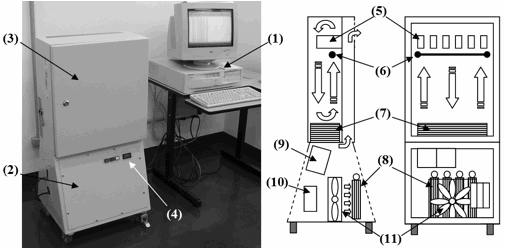
Figure 1. Test apparatus.
Using the described setup the key control elements are the on-off cycles to mimic the relays operation, the temperature control in the test chamber and the stress current (load) defined by the DC power supplies and the resistive loads, with their own cooling system (11) to keep stable the load conditions.
The apparatus is set up by installing 16 sample relays (5) and setting the heater (7) using its PID controller (4) to reach the testing temperature of 55oC in the test chamber. The on-off cycles are then started with relay number 1 using a square pulse of 100 ms, followed by an additional resting time of 100 ms. The switching square pulse follows cyclically to the remaining 15 relays until a new test cycle is restarted.
If a failure is detected the experiment controller stops the cycles and records the number of observed cycles with the associated failure mode, i.e., records an open or a closed-mode failure. After a faulty relay is detected it is removed from the experiment and its testing time of 200 ms is exchanged by a 120 ms dwell interval, decreasing the total cycle time from 3.2s to 2s when all but one relay has failed; see Table 1 for the minimum required time between successive operations. Notice also that the switching time of 100 ms is at least 3 times larger than the minimum switching time of 30 ms (Table 1) to create a safety margin to guarantee adequate relay operation.
3. Analysis and control of the test apparatus.
In the discussed experiment the temperature control in the test chamber, the experimental definition of stress levels and the detection of failures are the three main controlled variables to be analyzed.
The temperature control was implemented using the mentioned PID controller with an indicating accuracy of ± 1oC and continuous sampling interval of 500 ms. To close the control loop a J-type thermocouple (Figure 1-(6)) is used for a measuring accuracy of ± 0.4% of the nominal reading (ECIL, 2012), which gives ± 0.22 oC for the maximum working temperature (Table 1). The PID controller sets the heater on and off through a solid-state relay and creates an intermittent heat flow that warms up the content of the test chamber by convection, based on the feedback data from the thermocouple. With the adopted control scheme the temperature is kept nominally constant at 55oC in the test chamber when it is closed. After it is opened for relays removal a warm-up period of about 10 minutes needed to reestablish the testing temperature.
The stress levels are defined by choosing the appropriate resistive loads (Figure 1-(8)) using parallel associations of resistors as illustrated in Figure 2. Taking the DC power supplies of 24 ± 0.24 V with a total load capacity of 10 A, and assuming the multimeter measurement capability of ± (0.3% + 0.01) or ± 0.312 V for voltages, ±(0.4% + 0.02) or ± 0,360 A (max) for current and ±(0.4% + 0.2) or ± 0,800 Ω (max) for resistance, with a Uniform distribution for all multimeter readings, the resistors were measured and their combined uncertainties uc calculated according to the Guide to the expression of uncertainty in measurement (JCGM 100, 2008). The equivalent resistive loads Req given by equations (1) to (4) for the resistors associations illustrated in Figure 2, define the stress levels shown in Table 2 when the power supply of 24 V is used.
|
|
|
|
Stress 6A |
Stress 9 A |
Stress 12 A |
Stress 15 A |
Figure 2. Load resistors associations.
 (1)
(1)
 (2)
(2)
 (3)
(3)
 (4)
(4)
The resulting equivalent resistors Reqi are given in Table 3 for the nominal stresses of 6 A, 9 A, 12 A and 15 A respectively. Taking the individual resistors uncertainties uc, the combined uncertainties uc(Req) of the equivalent resistors Req were evaluated according to expressions (5) or (6) (JCGM 100, 2008), depending on whether they involved parallel or series associations. In expression (5), Ri,j stands for each individual resistor used in the associations (eq. 1 to 4) and uc(Ri,j) is the resulting combined uncertainty.
 (5)
(5)
 (6)
(6)
The resulting values of uc(Req) are also shown in Table 3.
Table 2 – Experimental definition of stress levels.
Nominal Stress [A] |
Req [W] |
uc(Req) [W] |
I [A] |
uc(I) [A] |
uc(I) [%] |
U(I) [A] |
6 |
3.922 |
0.010 |
6.12 |
0.034 |
0.56 |
0.068 |
9 |
2.600 |
0.012 |
9.25 |
0.063 |
0.68 |
0.126 |
12 |
2.073 |
0.012 |
11.60 |
0.088 |
0.76 |
0.176 |
15 |
1.572 |
0.009 |
15.27 |
0.116 |
0.76 |
0.232 |
Following the same reasoning the stress levels I and the associated combined uncertainties uc(I) were calculated according to expressions (7) and (8), were V is the voltage supply of 24 V and u(V) is the uncertainty of ± 0.24V from the power supply, here assumed as Normally distributed with a coverage factor K=2 (JCGM 100, 2008) based upon the manufacturer’s information.
![]() (7)
(7)
 (8)
(8)
Assuming uc(I) Normally distributed a coverage factor of K=2 can be used to derive in Table 2 the expanded uncertainties U(I). Table 2 also shows theproportion of uc(I) regarding the experimental values of I. It is important to highlight that the above uncertainties include all effects observed in the main components of the test apparatus, including the temperature variations during the resistance measurements and the set up of the test.
Regarding the elapsed time until failure, which is the life metrics for the tests, it is measured by a discrete variable that counts the number of cycles performed by each tested relay. The counting procedure is implemented in the PLC with the major concern of avoiding mistaken indications of individual failure modes, i.e., preventing the indication of an open-failure when a closed-failure is observed and vice-versa. The validation of failure mode indications was performed by conventional debugging in the PLC code and also by a cross checking procedure using a physical circuit that mimics the actual operation of tested relays.
Assuming the minimum switching of 30 ms given in Table 1 and the standard checking time of 100 ms for the PLC programming, a reference timer with accuracy of a few milliseconds was used to set operational times just above and below the 100ms marker. With a starting pulse a closed relay is commanded to open just before the PLC reaches its 100ms checking time. If it does not open a closed failure is recorded. A similar procedure is performed to command an opened relay to close just after 100 ms, when an opened failure is recorded. The reference timer is then used to vary command times below the 100 ms testing time and the cross checking is performed until it results in 100% of correct failure mode indication.
4. Test results and data analysis
Using the above-discussed experimental setup four groups of 16 samples were tested with the load currents I shown in Table 2. The test results are shown in Table 3 where the status ![]() indicates whether the associated time to failure
indicates whether the associated time to failure ![]() stands for a detected failure (F) or a censored sample (C). Each time to failure
stands for a detected failure (F) or a censored sample (C). Each time to failure ![]() shown in Table 3 refers to a single failure mode observed in each tested sample.
shown in Table 3 refers to a single failure mode observed in each tested sample.
Table 3 shows several censored readings when the stress of 6.12 A was used, while only one censored sample is observed for the stress of 9.25 A. The last two stress levels do not include censored samples and show reasonably closer values due to the similarity of relays’ behavior in these two stress levels.
Table 3 – Time to failure data.
Relay |
Stress level |
|||||||
6.12 A |
9.25 A |
11.60 A |
15.27 A |
|||||
|
|
|
|
|
|
|
|
|
1 |
480406 |
F |
73352 |
F |
31085 |
F |
45588 |
F |
2 |
551402 |
F |
98033 |
F |
98888 |
F |
111632 |
F |
3 |
813123 |
F |
236320 |
F |
109381 |
F |
113205 |
F |
4 |
1868621 |
C |
264699 |
F |
131948 |
F |
132499 |
F |
5 |
1868621 |
C |
420441 |
F |
132251 |
F |
153180 |
F |
6 |
1868621 |
C |
455503 |
F |
136459 |
F |
163699 |
F |
7 |
1868621 |
C |
495202 |
F |
138240 |
F |
164788 |
F |
8 |
1868621 |
C |
550119 |
F |
143818 |
F |
179237 |
F |
9 |
1868621 |
C |
733991 |
F |
191223 |
F |
204592 |
F |
10 |
1868621 |
C |
894067 |
F |
208244 |
F |
211918 |
F |
11 |
1868621 |
C |
953393 |
F |
209839 |
F |
216590 |
F |
12 |
1868621 |
C |
1793409 |
F |
229059 |
F |
251962 |
F |
13 |
1868621 |
C |
1817479 |
F |
254377 |
F |
266807 |
F |
14 |
1868621 |
C |
1882756 |
F |
433524 |
F |
300019 |
F |
15 |
1868621 |
C |
2064540 |
F |
500092 |
F |
367829 |
F |
16 |
1868621 |
C |
3309823 |
C |
522573 |
F |
526826 |
F |
5.1. The conventional ALT data analysis
Figure 3 organizes the conventional life-stress analysis (Nelson, 2004) in a nine-step procedure that starts with the collection of time-to-failure data as shown in Table 3 (step 1) in the form of ![]() .
.
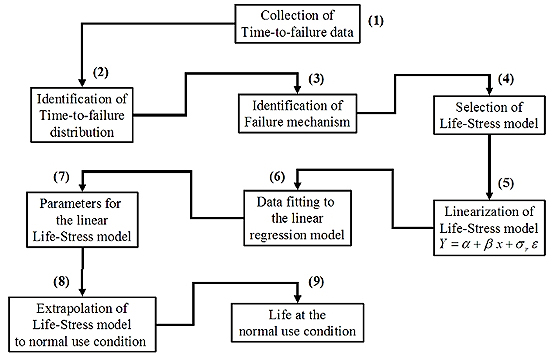
Figure 3. Life-stress analysis.
Step 2 deals with the identification of the appropriate time-to-failure distribution. This is done using a fitting method for the distribution parameters, capable of accounting for censored samples. In this case the Maximum Likelihood Estimator – MLE (Nelson, 2004) shown in expression (9) was used or the logarithmic of the Maximum Likelihood values in Table 4.
 (9)
(9)
Table 4 – Logarithmic of MLE values.
Stress Level [A] |
Distributions |
|||
Exponential |
Normal |
Log-Normal |
Weibull |
|
6.12 |
- 50.9408 |
- 52.4196 |
- 50.6077 |
- 50.9359 |
9.25 |
-223.2411 |
-229.1090 |
-222.8834 |
-223.2235 |
11.60 |
-212.5978 |
-212.3527 |
-209.6756 |
-209.8388 |
15.27 |
-212.3159 |
-208.6609 |
-207.0975 |
-207.2589 |
In the present discussion, the logarithmic transformations of MLE show maximum values of -50.6, -222.9, -209.7 and -207.1, pointing to the Log-Normal as the ideal distribution to model the collected time-to-failure data. The Log-Normal distribution is shown in expression (10), where s is the spread of the collected data and ![]() are the distribution parameters.
are the distribution parameters.
 (10)
(10)
Steps 3 and 4 are intended to identity the failure mechanism and to select the appropriate life-stress relationship. In this case the stress variable is the load current, which leads to a non-thermal stress in nature and allows selecting the Inverse-Power relationship shown in expression (11).
![]() (11)
(11)
In expression (11), I stands for the applied stress levels and ![]() are the parameters that represent the mechanism of failure, see Vassilou and Mettas (2002), Jayatilleka and Okogbaa (2003), Owen and Padget (2000) or Stepniak (1999) for details.
are the parameters that represent the mechanism of failure, see Vassilou and Mettas (2002), Jayatilleka and Okogbaa (2003), Owen and Padget (2000) or Stepniak (1999) for details.
In step 5 the selected life-stress relationship is linearized as illustrated in expressions (12) and (13), where![]()
![]() (12)
(12)
![]() (13)
(13)
The linear life-stress relationship given in (13) allows deriving the linear regression model shown in expression (14) (step 6) that is used in step 7 to calculate the parameters ![]() and
and![]() . In expression (14),
. In expression (14), ![]() is Normally distributed with zero mean (
is Normally distributed with zero mean (![]() ) and unitary variance (
) and unitary variance (![]() ). In the same expression
). In the same expression ![]() represents the expected variation due to the regression that must be independent of each stress levels.
represents the expected variation due to the regression that must be independent of each stress levels.
![]() (14)
(14)
Once the linear model is derived and the necessary parameters calculated using the collect experimental data, the life-stress relationship can be extrapolated (step 8) as indicated in expression (15) to generate life estimates ![]() (step 9) that represent the intended percentile.
(step 9) that represent the intended percentile.
![]() (15)
(15)
Following expression (15), the median life B50 and the B10 are calculated by making![]() and
and ![]() respectively (Nelson, 2004), as shown in Figure 4.
respectively (Nelson, 2004), as shown in Figure 4.
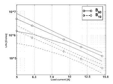
Figure 4. Conventional life-stress relationship.
Using the variance as given by expression (16) the associated 95% confidence limits can be calculated by expression (17).
![]() (16)
(16)
 (17)
(17)
Figure 4 highlights the estimated life at the nominal current of 5 A as recommended by the relay’s manufacturer (see Table 1), resulting in a median life B50 of 4959954 cycles. Its 95% confidence limit produces a lower bound of 1462674 cycles, which is roughly 46% larger than then minimum life expectation of 106 cycles given by the manufacturer (see Table 1). A similar analysis using the B10 estimator produces an estimated life of 1523221 cycles under normal conditions (5 A) with a lower bound of 443685 for its 95% confidence limit.
From the above discussion the motivation for the discussed experiment becomes explicit, since the measured life was reasonably larger than expected, even without considering the experimental uncertainty. A further analysis is then carried out to show the uncertainty influences on the obtained life estimates.
ALT data analysis under uncertainty conditions
To account for uncertainties in the experimental definition of stress levels a specialized procedure must be chosen, for which the SIMEX method (Cook and Stefanski, 1995) was selected; see Figure 5. This method allows estimating a set of parameters for a given regression model when the independent variable is subjected to measurement uncertainties. It offers normally asymptotic and consistent estimates for large or small samples, accounting for censored data with known or estimated variances, and disregarding the size of involved errors or uncertainties. The method is based upon the analysis of the trend created on the coefficients![]() ,
,![]() and
and ![]() (expression 14) when the independent variable (stress level) is influenced by controlled portions of uncertainties uc(I) [A] (Table 2).
(expression 14) when the independent variable (stress level) is influenced by controlled portions of uncertainties uc(I) [A] (Table 2).
In Figure 5 a coefficient ![]() in the range of
in the range of ![]() is sequentially taken to generate a Normally distributed samples of uncertainty values, that are used to derive new independent variables
is sequentially taken to generate a Normally distributed samples of uncertainty values, that are used to derive new independent variables ![]() as given in expression (18). The new life-stress relationship is shown in expression (19), which is derived from expression (14) once influenced by uncertainties.
as given in expression (18). The new life-stress relationship is shown in expression (19), which is derived from expression (14) once influenced by uncertainties.
![]() (18)
(18)
![]() (19)
(19)
A different stress level xn is then taken for each single value of ![]() and a large sample of
and a large sample of ![]() is generated to create distributions of
is generated to create distributions of ![]() ,
,![]() and
and![]() , whose mean values are used as the best estimates
, whose mean values are used as the best estimates![]() ,
, ![]() and
and ![]() for a chosen value of
for a chosen value of ![]() (see Figure 5). Once all
(see Figure 5). Once all![]() values are covered the functions
values are covered the functions![]() ,
,![]() and
and ![]() are obtained and the mentioned trend analysis is done using in the present case a quadratic model.
are obtained and the mentioned trend analysis is done using in the present case a quadratic model.
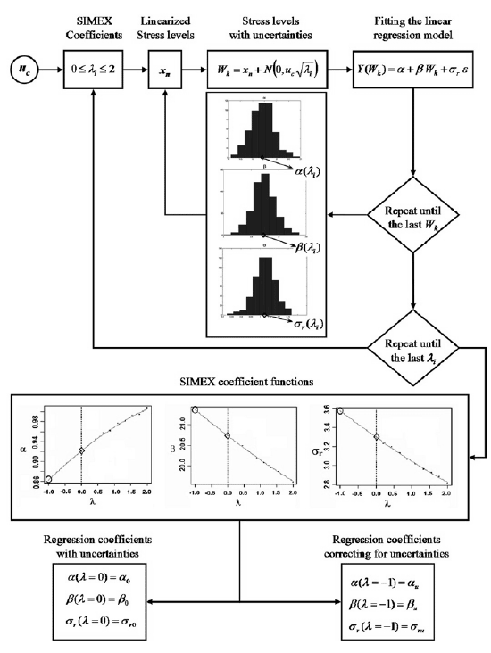
Figure 5. The SIMEX method.
In the described procedure the simulated uncertainty usimex are fractions of the combined uncertainties uc (Table 2) and are given by expression (20).
![]() (20)
(20)
The trend analysis is done by a regular curve fitting on functions ![]() ,
,![]() and
and ![]() to derive the extrapolated values of
to derive the extrapolated values of ![]() ,
, ![]() and
and ![]() when
when![]() , as shown in Figure 6.
, as shown in Figure 6.

Figure 6. The SIMEX coefficients a, b, dr.
Using ![]() ,
, ![]() and
and ![]() in expressions (15) and (17) the life estimates and the associated 95% confidence limits can be calculated to show the influence of uncertainties uc(I).
in expressions (15) and (17) the life estimates and the associated 95% confidence limits can be calculated to show the influence of uncertainties uc(I).
It is worth noticing that making![]() the uncertainty usimex = 0 in the extrapolation process and the SIMEX provides an estimated coefficients free of uncertainties; see expression (20) for details. Moreover, if
the uncertainty usimex = 0 in the extrapolation process and the SIMEX provides an estimated coefficients free of uncertainties; see expression (20) for details. Moreover, if ![]() in expression (20) the uncertainties u2simex becomes uc2(I) to provide a life estimate quite similar to the conventional data analysis, where the uncertainty is present in the experimental data but it is not accounted for in the coefficients calculations. Using the combined uncertainties of 0.034 A, 0.063 A, 0.088 A and 0.116 A given in Table 2 for the chosen stress levels, the SIMEX was used to derive life estimates at the intended normal use condition of 5 A.
in expression (20) the uncertainties u2simex becomes uc2(I) to provide a life estimate quite similar to the conventional data analysis, where the uncertainty is present in the experimental data but it is not accounted for in the coefficients calculations. Using the combined uncertainties of 0.034 A, 0.063 A, 0.088 A and 0.116 A given in Table 2 for the chosen stress levels, the SIMEX was used to derive life estimates at the intended normal use condition of 5 A.
Figure 6 illustrates the resulting functions ![]() ,
, ![]() and
and ![]() for the coefficients of expression (19). Although small in range, the plots clearly show the trend in the coefficients when
for the coefficients of expression (19). Although small in range, the plots clearly show the trend in the coefficients when ![]() is varied from 2.0 to -1.0 to account for uc(I) in the different stress levels. The extrapolation provides
is varied from 2.0 to -1.0 to account for uc(I) in the different stress levels. The extrapolation provides![]() ,
, ![]() and
and ![]() that is used in the linearized life-stress relationship to generate a B50 of 4963543 cycles with a lower bound of 1445852 cycles for the 95% confidence limit. A similar analysis generates a B10 estimate of 1524588 cycles with a lower bound of 444104 cycles. Table 5 summarizes the obtained results using the two discussed methods; i.e., the conventional analysis and the SIMEX method.
that is used in the linearized life-stress relationship to generate a B50 of 4963543 cycles with a lower bound of 1445852 cycles for the 95% confidence limit. A similar analysis generates a B10 estimate of 1524588 cycles with a lower bound of 444104 cycles. Table 5 summarizes the obtained results using the two discussed methods; i.e., the conventional analysis and the SIMEX method.
Table 5– Life estimates.
Method of analysis |
Corrections |
|||
Life estimate |
Conventional |
SIMEX |
Cycles |
(%) |
B50 |
4959954 |
4963543 |
3589 |
0.07 |
B50 lower limit |
1462674 |
1445852 |
-16821 |
-1.15 |
B10 |
1523221 |
1524588 |
1367 |
0.09 |
B10 lower limit |
443685 |
444104 |
419 |
0.09 |
The results show that having combined uncertainties uc(I) as small as 0.76% of the experimental current values (see Table 2) the SIMEX method provides absolute corrections for life estimates not greater than 1.15%, indicating that in this particular case the uncertainty influences were not significant.
However, having larger values of combined uncertainty, as usual in large scale experiments using shop floor instrumentation, the influences of uncertainties may increase to levels where it becomes relevant in accelerate life testing; see Figure 7.
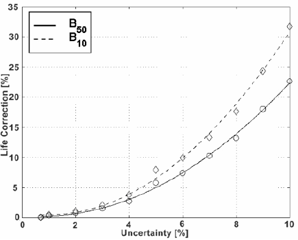
Figure 7. Effect of increasing uncertainties influences on life estimates.
Figure 7 shows the proportional corrections on life estimates when the uncertainty goes up to 10% of the experimental values of stress loads. The plot clearly shows that the corrections on life estimates systematically increase with uncertainties values, reaching 23 and 32 % for B10 and B50 respectively when the uncertainties increases to 10 % of the nominal values of stress loads. In Figure 7, the first point on the left depicts the data from Table 5 for the discussed experiment.
5. Conclusions
Regarding the test apparatus, the control upon the main influence variables provided the necessary validation of the experimental setup yielding the needed confidence on the results. The results seems adequate to the intended life investigation using an ALT approach, but the presence of measurement uncertainties pointed out another issue that needs further care depending on the available experimental resources.
Given the well-controlled conditions in the discussed experiment the influence of experimental uncertainties has proved not to be significant. However, the SIMEX results also show that the obtained estimates can be significantly affected if the experimental uncertainties are not kept below reasonable limits. Therefore, the actual significance of uncertainties in life estimates using accelerated life testing will depend upon the adopted experimental design, the test purpose and the test conditions.
Users of ALT must be aware about the presence of uncertainties in the experimental setup. Special attention should also be paid to the adopted methods for data analysis under uncertainty conditions.
Finally, the SIMEX method has proved to be robust and fully consistent with the discussed experiment even in the presence of censored data, small samples and uncertainties in the experimental setup. It provides a realistic measure of uncertainty influences from a practical point of view, allowing the analysis of a particular experimental setup to decide whether corrections on life estimates are needed. Such life estimates and the associated corrections can also be checked against actual performance data from products in the field to validate experimental approaches for ALT analysis in the log run.
Acknowledgments
The authors are thankful to Indústrias ROMI S.A., to the Universidade Metodista de Piracicaba - UNIMEP and to the Conselho Nacional de Desenvolvimento Científico e Tecnológico – CNPq for supporting this research.
References
Escobar, L. A.; Meeker, W. Q. (2006); “A review of accelerated test models”, Statistical Science, Vol. 21, No 4, pp. 552-577.
Huang, H. Z.; Liu, Z. J.; Murthy, D. N. P. (2007); “ Optimal reliability, warranty and price for new products”, IIIE Transactions, Vol. 39, No 8, pp. 819-827.
JCGM 100 (2008); “Evaluation of measurement data - Guide to the expression of uncertainty in measurement”,1st ed., Sèvres Cedex, France: Joint Committee for Guides in Metrology (JCGM). Bureau International des Poids et Mesures, 120p.
Sterl, R. (1997); Power relays, EH-Schrack Components AG, Vienna, Austria, 1997.
Wu, S. (2012); “Warranty data analysis: A Review”, Quality and Reliability Engineering International, Vol. 28, pp. 795-805.


